Classification of Functions
Functions are an essential part of mathematics, and understanding their classification can help us better grasp their properties and behavior. Today we will explore different ways functions can be classified based on their nature, behaviour, continuity, and injectivity/surjectivity.
1. Classification Based on the Nature of the Function
Functions can be classified based on their algebraic structure or how they are represented mathematically. We divide them into two main categories: Linear and Nonlinear. Nonlinear functions are further broken down into various subtypes.
a) Linear Functions
A linear function is of the form \(f(x) = mx + b\), where \(m\)and \(b\) are constants. These functions graph as straight lines.
Example: \(f(x) = 2x + 3\)
b) Nonlinear Functions
Nonlinear functions, unlike linear functions, do not form straight lines when graphed. These functions exhibit varying rates of change. There are several important subtypes of nonlinear functions, including polynomial, rational, exponential, and logarithmic functions.
i) Polynomial Functions
Polynomial functions are sums of terms, each of the form \(ax^n\), where \(a\) is a constant and \(n\) is a non-negative integer. They are generalized forms of linear and quadratic functions.
Example: \(f(x) = x^3 - 4x^2 + 5\)
ii) Quadratic Functions
A quadratic function is a second-degree polynomial of the form \(f(x) = ax^2 + bx + c\), where \(a \neq 0\). The graph of a quadratic function is a parabola.
Example: \(f(x) = x^2 + 3x + 2\)
ii) Rational Functions
A rational function is the ratio of two polynomials, i.e., \(f(x) = \frac{p(x)}{q(x)}\), where \(p(x)\)and \(q(x)\)are polynomials and \(q(x) \neq 0\).
Example: \(f(x) = \frac{x^2 - 1}{x + 2}\)
iii) Exponential Functions
An exponential function has the form \(f(x) = a^x\), where \(a\) is a positive constant. These functions grow (or decay) at an increasing rate.
Example: \(f(x) = 2^x\)
iv) Logarithmic Functions
A logarithmic function is the inverse of an exponential function and is of the form \(f(x) = \log_a(x)\), where \(a\) is the base of the logarithm.
Example: \(f(x) = \log_2(x)\)
2. Classification Based on the Behavior of the Function
Functions can also be classified based on certain properties such as symmetry and periodicity.
a) Even Functions
An even function is symmetric with respect to the y-axis, meaning that for every \(x\), \(f(x) = f(-x)\).
Example: \(f(x) = x^2\)
b) Odd Functions
An odd function has rotational symmetry about the origin, meaning that for every \(x\), \(f(x) = -f(-x)\).
Example: \(f(x) = x^3\)
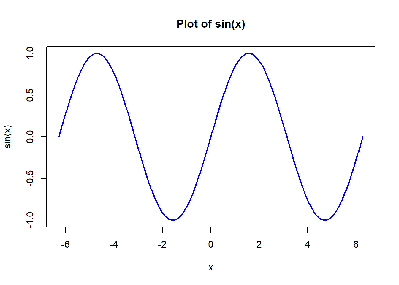
c) Periodic Functions
A periodic function repeats its values at regular intervals. The smallest such interval is called the period of the function.
Example: \(f(x) = \sin(x)\)
3. Classification Based on Continuity
Functions can be classified based on whether they are continuous or discontinuous.
a) Continuous Functions
A function is continuous if it has no breaks, jumps, or holes in its graph. More formally, a function \(f(x)\)is continuous at a point \(x = a\) if:
\[ \lim_{x \to a} f(x) = f(a) \]
Example: \(f(x) = x^2\)
b) Discontinuous Functions
A discontinuous function has one or more points where it is not continuous, such as jumps, holes, or asymptotes.
Example: \(f(x) = \frac{1}{x}\)
4. Piecewise-Defined Functions
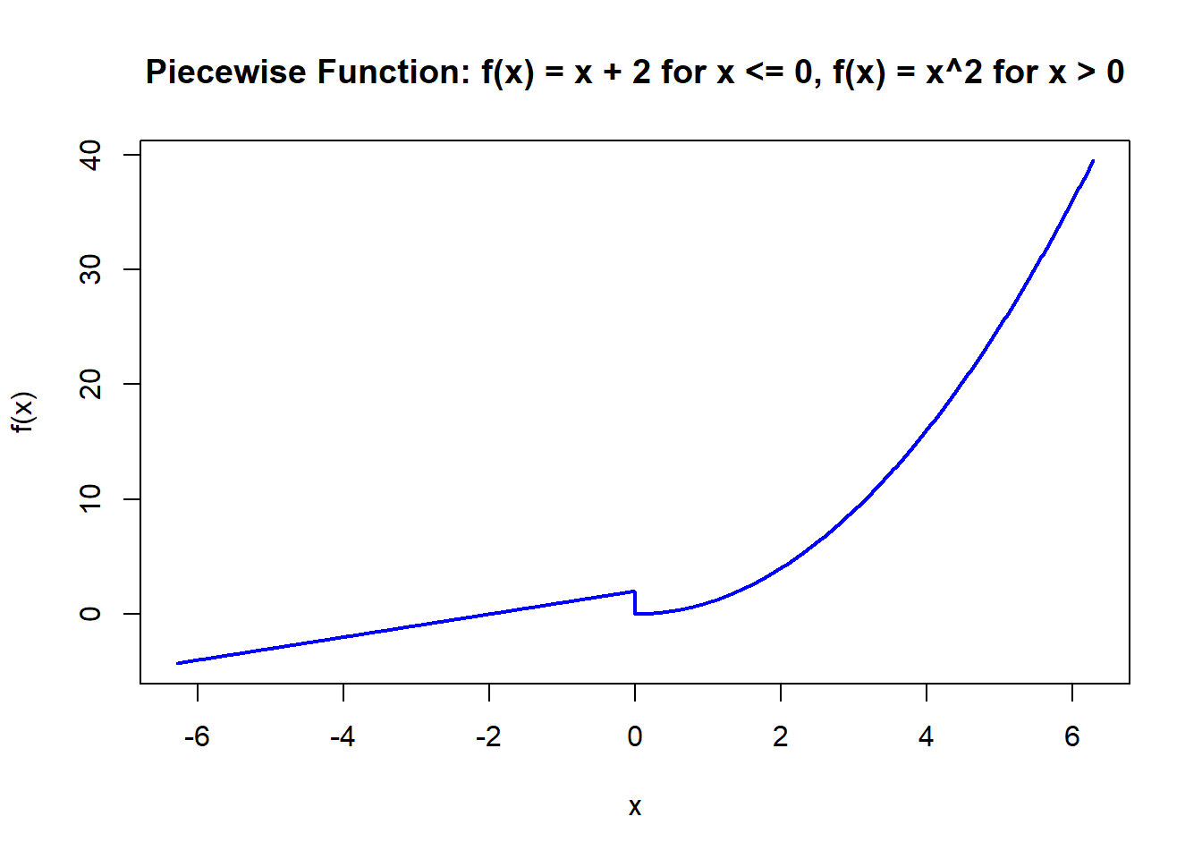
Sometimes an equation can’t be described by a single equation, and instead, we need to describe it using a combination of equations. Such functions are called piecewise-defined functions. The easiest way to describe piecewise-defined functions is to look at a couple of examples.
Piecewise-defined functions are functions that are described by different expressions over different parts of their domain. In other words, for different intervals of \(x\), the function behaves according to a different equation.
Example 1: A simple example of a piecewise function is:
\[ f(x) = \begin{cases} x + 2, & \text{if } x \leq 0 \\ x^2, & \text{if } x > 0 \end{cases} \] In this function:
- For \(x \leq 0\), the function behaves like a linear function \(f(x) = x + 2\).
- For \(x > 0\), the function behaves like a quadratic function \(f(x) = x^2\).
This combination of linear and quadratic functions defines the behavior of \(f(x)\) over different intervals.

Example 2: Another example could be a piecewise function that combines absolute value and a constant:
\[ g(x) = \begin{cases} |x|, & \text{if } x < 0 \\ 5, & \text{if } x \geq 0 \end{cases} \]
Here:
- For \(x < 0\), the function takes the form of the absolute value function \(g(x) = |x|\).
- For \(x \geq 0\), the function is constant, \(g(x) = 5\).
Piecewise functions are particularly useful for modeling situations where different behaviors occur under different conditions. They provide a way to describe real-world scenarios where a function changes its rule depending on the input.
Note: There are other classification, such as those based on injectivity and surjectivity, but they are beyond the scope of this course.
Thank you for visiting! Explore the other pages for more insights and resources.